When researching data we want to find features that help us understand the information. We look for insight in areas like Machine Learning or other fields in Mathematics and Artificial Intelligence. I want to present here a tool initially coming from Mathematics that can be used for exploratory data analysis and give some geometric insight before applying more sophisticated algorithms.
The tool I want to describe is Persistent Homology, member of a set of algorithms known as Topological Data Analysis. In this post I will describe the basic methodology when facing a common data analysis scenario: clustering.
SOME IDEAS FROM TOPOLOGY
A space is a set of data with no structure. The first step is to give some structure that can help us understand the data and also make it more interesting. If we define a notion of how close are all the points we are giving structure to this space. This notion is a neighborhood and it tells us if two points are close. With this notion we already have important information: we now know if our data is connected.
The neighborhoods can be whatever we want and the data points can be numbers or words or other type of data. These concepts and ideas are the subject of study of Topology. For us, Topology is the study of the shape of data.
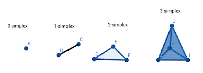
We need to give some definitions, but all are very intuitive. From our point space or dataset, we define the following notion: a simplex. It is easy to visualize what we mean.
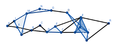
So, a 0-simplex is a point. Every point in our data is a 0-simplex. If we have a “line” joining two points that is a 1-simplex, and so on. Of course, a 4-simplex and higher analogues are difficult for us to visualize. We can immediately see what connectedness is. In the image, we have four connected components, a 0-simplex, a 1-simplx, a 2-simplex and a 3-simplex. If we join them with, for example lines we will connect the dataset into one single component. Like this:
The next notion is the neighborhood. We’ll use euclidean distance to say when our points are close, we’ll use circles as neighborhoods. This distance depends on a parameter, the radius of the circle. If we change these parameter we change the size of the neighborhood.
Persistence is an algorithm that changes this parameter from zero to a very large value, one that covers the entire set. With this maximal radius we enclose all our dataset. The algorithm can be put as follows:
1. We construct a neighborhood for each point and set the parameter to zero.
2. Increment the value of this parameter and if two neighborhoods intersect, draw a line between the points. These will form a 1-simplex. After that an n-simplex will form at each step until we fill all the space with lines.
3. Describe in some way the holes of our data has as we increase the parameter. Keep track when they emerge and when they disappear. If the holes and voids persist as we move the parameter, we can say that we found an important feature of a our data
The “some way” part is called Homology and is a field in Mathematics specialized in detecting the structure of space. The reader can refer to the bibliography for these concepts.
This algorithm can be shown to detect holes and voids in datasets. An achievement we can mention is that Persistent Homology was used for detecting a new subtype of breast cancer using it to detect clusters in images.
We will use R language integrated with the SAP HANA database to work with these tools.
VEHICLE DATASET
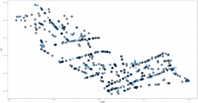
The dataset is available in. It’s about car accidents and has some specifications. We query in HANA only the data we need for this demo. We use an ID of the accident, the spatial coordinates and categorical data: Local highway authority and Road Type. That’s all we need to start. This data looks like this:
Then we visualize this data:
Now we use the Topological Data Analysis library in the R language for study the data. And store the information to make a visualization later.
DROP PROCEDURE "TDA";
-- procedure with R script using TDA package
CREATE PROCEDURE "TDA" (IN vehic_data "VEHIC_DATA", OUT persistence "PERSISTENCE")
LANGUAGE RLANG AS
BEGIN
library(TDA)
persist <- function(vehic_data){
#We point out that the columns are only the spatial coordinates
#You can find how to construct this example in TDA package documentation
vehic_vector <- cbind("V1" = vehic_data$longitude, "V2" = vehic_data$latitude)
xlimit <- c(-0.3, 0)
ylimit <- c(51.2, 51.6)
by <- 0.002
x_step <- seq(from = Xlim[1], to = Xlim[2], by = by)
y_step <- seq(from = Ylim[1], to = Ylim[2], by = by)
grid <- expand.grid(x_step, y_step)
diag <- gridDiag(X = vehic_vector, FUN = distFct, lim = cbind(xlimit, ylimit), by = by,
sublevel = FALSE, library = "Dionysus", printProgress = FALSE)
# Since gridDiag returns a list, we access this in any way we want:
diagram <- Diag[["diagram"]]
topology <- data.frame(cbind("dimension"=a[,1],"death"=a[,2],"birth"=a[,3]))
return(topology)
}
# Use the function
persistence <- persist(vehic_data)
END;
-- call to keep results in a table
CALL "TDA" ("VEHIC_DATA", "PERSISTENCE") WITH OVERVIEW;
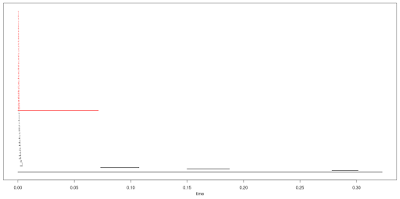
Next we visualize the results. Here I show you the results in R, using package TDA itself, just as an example.
This is a Barcode. The barcode shows the persistence of some topological features of our data vs the parameter “time”, this is the radius of our neighborhoods as we increase it. The red line tells us that there is a “hole”, an empty space, and we can check this in the visualization. The other lines represent connected components of the dataset, this means we have clustering. The barcode shows that we can expect 3 or 4 important clusters that will persist even if the data has noise.
The ability to persist is a topological property of the data.
After this analysis, we can start the usual Machine Learning approach: K-means…
Since this data was too dense in its parameters, we have to use other settings in Topological Data Analysis to find better approximations to the persistent characteristics. Euclidean distance only help us as a start, we can change this to more specialized filtering of our data. But we can be sure we have a good approximation, Persistence Homology is robust against noise and smooth changes in the data.
We will explore some of these ideas in the next blogs and compare to the usual approaches in Machine Learning.


