Read on if you want to know how R syntax can be deployed in SAP Data Hub. I will use time series forecasting to introduce this concept. Think of demand forecasting or sales forecasting, just to give a few examples for how this might be used in a business context.
Generally, you can choose from a number of technologies for time series forecasting. You can select a highly automated approach (ie with SAP Predictive Analytics), you can leverage conventional algorithms inside SAP HANA (Predictive Analytics Library) or you can bring in open source such as R or Python.
This blog explains how to implement such a requirement with R in SAP Data Hub. Just note that there is also an option to implement R syntax directly in a SAP HANA procedure.
SAP Data Hub however provides additional functionality that can be very useful in deploying predictive models. It can combine heterogenous data sources and transform or enrich the data in a graphical flowchart. It is also providing data governance and a scheduling mechanism.
In this blog we will forecast how many passenger vehicles will be registered in the next 12 months in a number of European countries. This is the same use case and data as used in the earlier blog on SAP HANA procedures.
Disclaimer: I should point out that any code or content in this blog is not supported by SAP and that you have to validate any code or implementation steps yourself.
Just reading this blog will hopefully give you a good idea for how R syntax can be leveraged in SAP Data Hub. Should you want to implement the example yourself, you must have access to
◈ SAP Data Hub (this blog is written with version 2.3, earlier versions will not suffice)
◈ SAP HANA as data source and target (no R server has to be connected to this SAP HANA)
◈ R editor (ie RStudio) to develop the script
◈ SAP HANA Client to allow the R editor to connect to SAP HANA
The SAP Data Hub 2.3 trial currently does not include a SAP HANA image. If you are using this trial, you need to combine it with a separate SAP HANA instance.
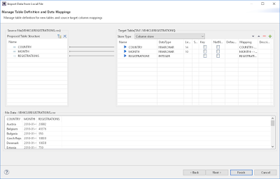
Start by loading the historic data into SAP HANA. Use your preferred option to load the content of VEHICLEREGISTRATIONS.csv into a table. If you are using the SAP HANA Modeler, you can choose: File → Import → SAP HANA Content → Data from Local File. I am loading the data into the table TA01.VEHICLEREGISTRATIONS.
Generally, you can choose from a number of technologies for time series forecasting. You can select a highly automated approach (ie with SAP Predictive Analytics), you can leverage conventional algorithms inside SAP HANA (Predictive Analytics Library) or you can bring in open source such as R or Python.
This blog explains how to implement such a requirement with R in SAP Data Hub. Just note that there is also an option to implement R syntax directly in a SAP HANA procedure.
SAP Data Hub however provides additional functionality that can be very useful in deploying predictive models. It can combine heterogenous data sources and transform or enrich the data in a graphical flowchart. It is also providing data governance and a scheduling mechanism.
In this blog we will forecast how many passenger vehicles will be registered in the next 12 months in a number of European countries. This is the same use case and data as used in the earlier blog on SAP HANA procedures.
Disclaimer: I should point out that any code or content in this blog is not supported by SAP and that you have to validate any code or implementation steps yourself.
Prerequisites
Just reading this blog will hopefully give you a good idea for how R syntax can be leveraged in SAP Data Hub. Should you want to implement the example yourself, you must have access to
◈ SAP Data Hub (this blog is written with version 2.3, earlier versions will not suffice)
◈ SAP HANA as data source and target (no R server has to be connected to this SAP HANA)
◈ R editor (ie RStudio) to develop the script
◈ SAP HANA Client to allow the R editor to connect to SAP HANA
The SAP Data Hub 2.3 trial currently does not include a SAP HANA image. If you are using this trial, you need to combine it with a separate SAP HANA instance.
Load historic data into SAP HANA
Start by loading the historic data into SAP HANA. Use your preferred option to load the content of VEHICLEREGISTRATIONS.csv into a table. If you are using the SAP HANA Modeler, you can choose: File → Import → SAP HANA Content → Data from Local File. I am loading the data into the table TA01.VEHICLEREGISTRATIONS.
Develop R script for forecasting
Use your preferred R editor to script the forecasting code you want to deploy later on in SAP Data Hub. To help scalability develop a script that forecasts only one single time series. SAP Data Hub will be able to apply this script on as many time series as needed.
As such download the history of only a single time series into your R editor. A quick method to connect would be to pass the logon parameters through code.
library("RJDBC")
jdbc_driver <- JDBC(driverClass = "com.sap.db.jdbc.Driver",
classPath = "C:/Program Files/SAP/hdbclient/ngdbc.jar")
jdbc_connection <- dbConnect(jdbc_driver,
"jdbc:sap://SERVER:PORT",
"YOURUSER",
"ANDYOURPASSWORD")
data <- dbGetQuery(jdbc_connection, "SELECT COUNTRY, MONTH, REGISTRATIONS FROM TA01.VEHICLEREGISTRATIONS WHERE VEHICLEREGISTRATIONS.Country = 'United Kingdom' ORDER BY MONTH ASC")
However, it is not elegant to have the password visible in your code. It would be better to save the logon parameters securely with the hdbuserstore application, which is part of the SAP HANA client.
Navigate in a command prompt to the folder that contains the hdbuserstore, ie
C:\Program Files\SAP\hdbclient
Then store the logon parameters in the hdbuserstore. In this example the parameters are saved under a key that I called myhana.
C:\Program Files\SAP\hdbclient>hdbuserstore -i SET myhana “SERVER:PORT” YOURUSER
And now the logon in R is much slicker.
library(RJDBC)
jdbc_driver <- JDBC(driverClass = "com.sap.db.jdbc.Driver",
classPath = "C:/Program Files/SAP/hdbclient/ngdbc.jar")
jdbc_connection <- dbConnect(jdbc_driver, "jdbc:sap://?key=myhana")
data <- dbGetQuery(jdbc_connection, "SELECT COUNTRY, MONTH, REGISTRATIONS FROM TA01.VEHICLEREGISTRATIONS WHERE VEHICLEREGISTRATIONS.Country = 'United Kingdom' ORDER BY MONTH ASC")
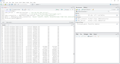
In that R code we are already retrieving the history of the first time series. I just chose the history of the United Kingdom. It could have been any other. Now that the data is in R, you are free to script your preferred forecasting logic. I will be using the following function, which I called forecast_monthly(). That function makes use of a few R libraries. You may have to add these to your system with the usual install.packages() function.
forecast_monthly <- function(data){
# Load required libraries ---------------------------------------------------------
library(lubridate)
library(forecast)
library(MLmetrics)
# Specify any parameters, adjust to the use case ----------------------------------
col_name_date <- "MONTH"
col_name_measure <- "REGISTRATIONS"
col_name_segment <- "COUNTRY"
date_format <- "%Y-%m-%d"
dates_to_forecast <- 12
confidence_level <- 0.95
forecast_methods <- c('arima', 'ets', 'rwdrift', 'naive')
frequency <- 12 # This value must not be changed
# Retrieve the individual columns from the data frame -----------------------------
col_date <- as.character(data[, col_name_date])
col_measure <- data[, col_name_measure]
col_segment <- data[1, col_name_segment]
# Print status update -------------------------------------------------------------
print(paste("Now starting with: ", col_segment, sep = ""))
# Ensure data is sorted on the date in ascending order ---------------------------
data <- data [order(data[, col_name_date]), ]
# Convert time series into ts object (required by forecast function) --------------
start_date <- as.Date(data[1, col_name_date], date_format)
ts_historic <- ts(data[, col_name_measure],
start = c(year(start_date), month(start_date)),
frequency = frequency)
# Keep a hold out sample of forecast length to test forecast accuracy -------------
ts_short <- head(ts_historic, n = length(ts_historic)-dates_to_forecast)
ts_hold_out <- tail(ts_historic, n = dates_to_forecast)
# Assess all forecasting methods on their performance on the hold out sample ------
ts_short_mapes <- rep(NA, length(forecast_methods))
for (ii in 1:length(forecast_methods)) {
stlf_forecast <- stlf(ts_short,
method = forecast_methods[ii],
h = dates_to_forecast,
level = confidence_level)
ts_short_mapes[ii] <- MAPE(as.numeric(ts_hold_out), stlf_forecast$mean)
}
# Select the best performing method to carry out the final forecast ---------------
forecast_best_mape <- min(ts_short_mapes)
ts_forecast <- stlf(ts_historic,
method = forecast_methods[which(ts_short_mapes == forecast_best_mape)],
h = dates_to_forecast,
level = confidence_level)
# Dates, name of time series (segment) and date type (Actual or Forecast) ---------
dates_all <- as.character(seq(from = start_date, by = "month", length.out = length(ts_historic)+dates_to_forecast))
col_segments <- rep(col_segment, length(dates_all))
model_descr <- rep(paste(ts_forecast$method, "- MAPE:", round(forecast_best_mape, 3)), length(dates_all))
date_types <- as.character(c(rep("Actual", length(ts_historic)), rep("Forecast", dates_to_forecast)))
# Actual and historic measures ----------------------------------------------------
forecast_mean <- rep(NA, dates_to_forecast)
forecast_mean <- ts_forecast$mean
forecast_upper <- ts_forecast$upper
forecast_lower <- ts_forecast$lower
dates_all_mean <- as.numeric(c(as.numeric(ts_historic), as.numeric(forecast_mean)))
dates_all_lower <- as.numeric(c(rep(NA, length(ts_historic)), as.numeric(forecast_lower)))
dates_all_upper <- as.numeric(c(rep(NA, length(ts_historic)), as.numeric(forecast_upper)))
# Return the combined data --------------------------------------------------------
result <- data.frame(SEGMENT = col_segments,
MONTH = dates_all,
MEASURETYPE = date_types,
MEASURE = dates_all_mean,
MEASURELOWER = dates_all_lower,
MEASUREUPPER = dates_all_upper,
MODEL = model_descr)
return(result)
}
Define the function and call it by passing the historic data of a single country as parameter.
library(RJDBC)
jdbc_driver <- JDBC(driverClass = "com.sap.db.jdbc.Driver",
classPath = "C:/Program Files/SAP/hdbclient/ngdbc.jar")
jdbc_connection <- dbConnect(jdbc_driver, "jdbc:sap://?key=myhana")
data <- dbGetQuery(jdbc_connection, "SELECT COUNTRY, MONTH, REGISTRATIONS FROM TA01.VEHICLEREGISTRATIONS WHERE VEHICLEREGISTRATIONS.Country = 'United Kingdom' ORDER BY MONTH ASC")
forecast_monthly(data)
You should then see the output of the function, which contains both the historic data as well as the forecast for the next 12 months. This function will be deployed through SAP Data Hub.
Create target table in SAP HANA
When forecasting the demand through SAP Data Hub the predictions can be written into a SAP HANA table. Execute the following SQL syntax in SAP HANA to create a table that matches the output structure of the forecast_monthly() function, so that it can store the predictions.
SAP Data Hub version 2.3 does not support columns of type DECIMAL, use DOUBLE instead.
SET SCHEMA TA01;
--- Create table for the output
DROP TABLE "VEHICLEREGISTRATIONS_FORECAST";
CREATE COLUMN TABLE "VEHICLEREGISTRATIONS_FORECAST"(
SEGMENT NVARCHAR(14),
MONTH DATE,
MEASURETYPE NVARCHAR(20),
MEASURE DOUBLE,
MEASURELOWER DOUBLE,
MEASUREUPPER DOUBLE,
MODEL NVARCHAR(100));
Now everything is in place to deploy the forecasting script in SAP Data Hub. The major steps in implementing the full deployment are
◈ Obtain a list of all countries that need to be forecasted
◈ For each country obtain the individual history
◈ Create an individual forecast for each country
◈ Write each forecast to SAP HANA
Connect SAP Data Hub to SAP HANA
First establish a connection from SAP Data Hub to SAP HANA. Open the SAP Data Hub in your browser and go into the Connection Management.
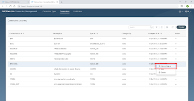
Create a new connection to your SAP HANA system, using the connection type HANA_DB. The remaining settings are rather straight-forward. Specify the SAP HANA host, the port and your logon credentials. You can keep the remaining default settings. I have named my connection MYHANA.
Once the connection is created, test whether it is working well. On the overview page that lists all connection, click on the three little dots to the right-hand side of your connection. Select “Check Status” and you should get a confirmation message.
Obtain list of all countries
We want to create a forecast for each country that is found in the historic data. That dynamic approach helps reduce maintenance efforts. We will use a SELECT statement to retrieve that list. On SAP Data Hub’s main page click into the “Modeler”, which is where you create the graphical pipeline.
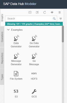
In the menu on the left you see different tabs. The “Graphs” section is showing is showing some examples of pipelines. The “Operators” section contains a long list of graphical operators you can combine in a graph.
Make sure you are on the “Graphs” section, then create a new Graph with the plus sign on top. An empty canvas opens up. I prefer to give it a name right away. Click the save symbol on top and name it “R_Forecasting”.
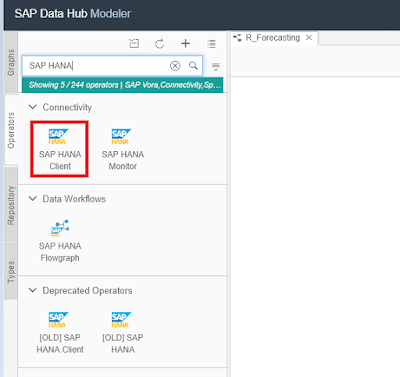
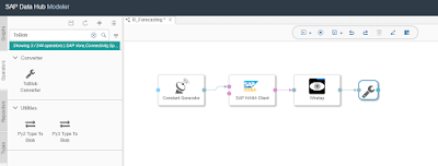
To obtain a list of the countries that need to be forecasted, add a “SAP HANA Client” operator to the graph. Select the “Operators” section on the left and search for SAP HANA. The SAP HANA Client shows up.
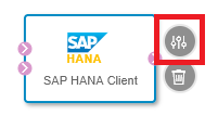
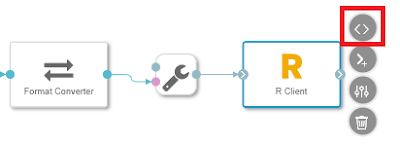
Drag the icon onto the empty canvas. Open it’s configuration panel by clicking the symbol on its right hand side.
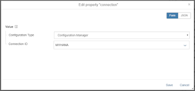
On the configuration panel you just need to open the graphical Connection editor by clciking on the small icon to the right of “Connection”. Set the “Configuration Type” to “Configuration Manager” and you can select the name of the connection you had created earlier in the “Connection Management”, then Save.
Now this SELECT statement needs to be passed to the SAP HANA Client to get the desired list.
SELECT DISTINCT COUNTRY FROM TA01.VEHICLEREGISTRATIONS;
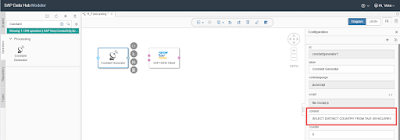
This is done with the Operator called “Constant Generator”. Add such an operator to the left of the SAP HANA Client. Open the Constant Generator’s configuration panel. Paste the above statement into the content configuration.
To connect the two operators click the output port of the “Constant Generator” and drag the mouse onto the sql input port of the SAP HANA Client.
Add a “Wiretap” Operator to the output of the SAP HANA Client. This will allow us to see the data that was retrieved from SAP HANA.
Save the Graph and start it by clicking the “Run” button on top.
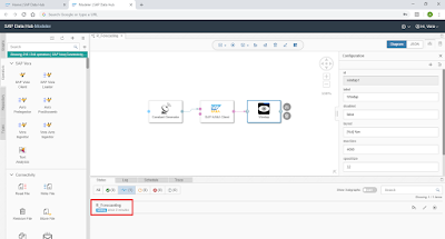
And if all goes well, the graph should briefly show at the bottom of the screen as pending graph, before moving to the running graphs section. We will see later how to terminate such a graph after its completion. To see the records that were retrieved from SAP HANA, click on the running graph at the bottom of the screen.
A new page opens, showing the current status of the running graph. On this screen, open the Wiretap’s User Interface.
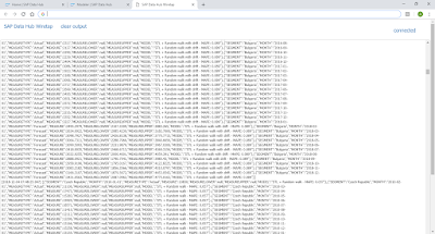
A separate Browser tab opens and displays the retrieved data in message format.
Now terminate this graph with the “Stop Process” button at the bottom of the modeler page.
Obtain each country’s individual history
To retrieve the history of each country, the appropriate individual SELECT statements have to be created and sent to a second SAP HANA Client. We will use JavaScript to access the different Countries in the output of the first SAP HANA Client to create the correct SELECT statements.
When we come to the JavaScript syntax we want to have the input data in JSON format. SAP Data Hub comes with an operator that turns a blob into JSON format. As our data is in message format, first add a “ToBlob Converter”, so that we can use the converter to JSON format.
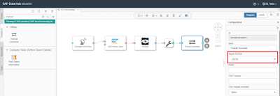
Now we can add the “Format Converter”, which produces JSON output by default.
Now add a “ToString Converter” to the end of the graph, which is needed for the JavaScript operator to read the data correctly. Connect the Format Converter’s output to the lower input port of the ToString operator.
By the way, in case your graph does not look as orderly, you can click the “Auto Layout” button on top to get the icons in line.
Now on the Modeler’s Operator tab search for JavaScript and add the “Blank JavaScript” operator to the graph.
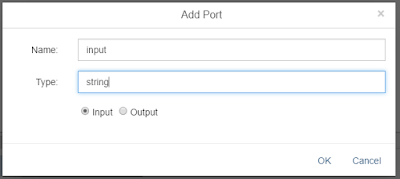
This operator does not have any input or output ports yet. These can be manually added. Right click the new operator and select “Add Port”. The JSON data will be retrieved as string. Hence name the first port “input” with Type “string”. Keep the radio button on “Input”.
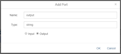
The JavaScript will output SELECT statements in string format. Hence create a second port. Name it “output”, with Type “string” and switch the radio button to “Output”.
Now you can connect the ToString’s output port to the JavaScript’s input port. Then open the new node’s Script setting.
Copy the following code into the Script window. The first line specifies that the onInput function will be called when data is retrieved on the “input” port. The onInput function retrieves the input data and parses the JSON format. It then iterates through all countries and outputs for each country the SELECT statement that requests each country’s history.
$.setPortCallback("input",onInput)
function onInput(ctx,s) {
var json = JSON.parse(s);
for(var ii = 0; ii < json.length; ii++) {
var country_name = json[ii].COUNTRY;
$.output("SELECT COUNTRY, MONTH, REGISTRATIONS FROM TA01.VEHICLEREGISTRATIONS WHERE VEHICLEREGISTRATIONS.COUNTRY = '" + country_name + "' ORDER BY MONTH ASC;")
}
}
Close the Script window with the small cross on top.
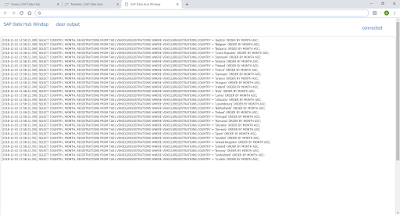
Connect a second Wiretap operator to the output of the JavaScript operator. Save and run the graph. In the Wiretap’s UI you see the SELECT statements coming from the JavaScript’s output port.
These SELECT statements now need to be passed to a SAP HANA Client to execute them. This is now very much the same as what we had at the very start of this graph. Add a SAP HANA Client, specify its connection and add a Wiretap to the end to verify the output.
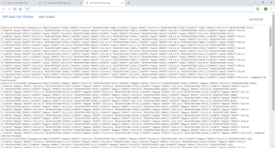
Run the graph and in the Wiretap UI you see the history of each country. Each country is an individual request, which allows SAP Data Hub to scale the operation. Note that by default the Wiretap is showing only the first 4092 characters. Hence not all countries show up. This value can be increased though in the Wiretap’s configuration.
Create the forecasts in R
We now have the input data needed for our time series forecasts. Before continuing with the graph however, we need to provide a Docker file, which SAP Data Hub can use to create Docker containers to run the R syntax in.
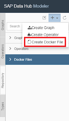
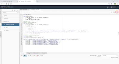
Go into the “Repository” tab on the Modeler menu. Click the plus-sign on top and choose “Create Docker File”.
Name it “Docker_R_Forecast”. The following Docker syntax worked well for me. It is installing for example the forecast package which is carrying out the predictions in our code. Copy and paste this into the Docker file. Adjust it as you see fit.
FROM debian:9.4
RUN apt-get update \
&& apt-get install -y --no-install-recommends \
locales \
&& rm -rf /var/lib/apt/lists/*
## Install R
## Set a default CRAN repo
RUN apt-get update \
&& apt-get install -y --no-install-recommends \
r-base \
r-base-dev \
r-recommended \
libnlopt-dev \
curl \
&& echo 'options(repos = c(CRAN = "https://cran.rstudio.com/"), download.file.method = "libcurl")'>> /etc/R/Rprofile.site \
&& rm -rf /tmp/downloaded_packages/ /tmp/*.rds \
&& rm -rf /var/lib/apt/lists/*
## Install additional R packages
RUN apt-get update
RUN apt-get install libcurl4-openssl-dev
RUN echo 'options(repos="https://cran.rstudio.com/", download.file.method = "libcurl")'>> /etc/R/Rprofile.site \
&& Rscript -e "install.packages(c('Rserve'), dependencies=TRUE)" \
&& Rscript -e "install.packages(c('jsonlite'), dependencies=TRUE)" \
&& Rscript -e "install.packages(c('MLmetrics'), dependencies=TRUE)" \
&& Rscript -e "install.packages(c('forecast'), dependencies=TRUE)" \
&& Rscript -e "install.packages(c('lubridate'), dependencies=TRUE)"
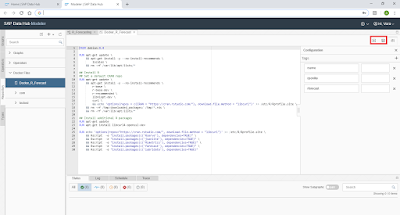
Open the Docker file’s configuration with the icon on the top right corner.
This opens a side panel, in which we need to enter some tags. These tags help SAP Data Hub to start the most appropriate Docker container for your code. Add the tags rserve and rjsonlite, should they already exist. Then add a new tag, let’s call it rforecast to indicate that this Docker file is installing the packages needed for our forecasting. Then save the file and initiate the Docker build with the icon right next to it.
The build process might take half an hour or longer.
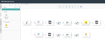
Go back to the graph, where we need to transform the data again into JSON format, just like before. Add a ToBlob Converter, followed by a Format Converter, followed by a ToString Converter.
This brings the data into the format that R can process it. Add an R Client operator.
The operator does not have any ports yet. As before, create an input port named “input” of type string, and an output port named “output” also of type string. Then connect the R Client with the previous node. Open the R Client’s Script window.
Delete the default script and paste the following R code inside. The first line specifies that the dh_forecast() function is called when data arrives. This function is transforming the input data from JSON to a data frame before passing the data to the forecast_monthly() function we have already used in the R Editor. The output of the forecast_monthly() function is then transformed into JSON format before passing the data to the output port. Close the script window.
api$setPortCallback(c("input"), c("output"), "dh_forecast")
dh_forecast <- function(data) {
data <- fromJSON(data)
result <- forecast_monthly(data)
result <- toJSON(result, na = 'null')
list(output=result)
}
forecast_monthly <- function(data){
# Load required libraries ---------------------------------------------------------
library(lubridate)
library(forecast)
library(MLmetrics)
# Specify any parameters, adjust to the use case ----------------------------------
col_name_date <- "MONTH"
col_name_measure <- "REGISTRATIONS"
col_name_segment <- "COUNTRY"
date_format <- "%Y-%m-%d"
dates_to_forecast <- 12
confidence_level <- 0.95
forecast_methods <- c('arima', 'ets', 'rwdrift', 'naive')
frequency <- 12 # This value must not be changed
# Retrieve the individual columns from the data frame -----------------------------
col_date <- as.character(data[, col_name_date])
col_measure <- data[, col_name_measure]
col_segment <- data[1, col_name_segment]
# Print status update -------------------------------------------------------------
print(paste("Now starting with: ", col_segment, sep = ""))
# Ensure data is sorted on the date in ascending order ---------------------------
data <- data [order(data[, col_name_date]), ]
# Convert time series into ts object (required by forecast function) --------------
start_date <- as.Date(data[1, col_name_date], date_format)
ts_historic <- ts(data[, col_name_measure],
start = c(year(start_date), month(start_date)),
frequency = frequency)
# Keep a hold out sample of forecast length to test forecast accuracy -------------
ts_short <- head(ts_historic, n = length(ts_historic)-dates_to_forecast)
ts_hold_out <- tail(ts_historic, n = dates_to_forecast)
# Assess all forecasting methods on their performance on the hold out sample ------
ts_short_mapes <- rep(NA, length(forecast_methods))
for (ii in 1:length(forecast_methods)) {
stlf_forecast <- stlf(ts_short,
method = forecast_methods[ii],
h = dates_to_forecast,
level = confidence_level)
ts_short_mapes[ii] <- MAPE(as.numeric(ts_hold_out), stlf_forecast$mean)
}
# Select the best performing method to carry out the final forecast ---------------
forecast_best_mape <- min(ts_short_mapes)
ts_forecast <- stlf(ts_historic,
method = forecast_methods[which(ts_short_mapes == forecast_best_mape)],
h = dates_to_forecast,
level = confidence_level)
# Dates, name of time series (segment) and date type (Actual or Forecast) ---------
dates_all <- as.character(seq(from = start_date, by = "month", length.out = length(ts_historic)+dates_to_forecast))
col_segments <- rep(col_segment, length(dates_all))
model_descr <- rep(paste(ts_forecast$method, "- MAPE:", round(forecast_best_mape, 3)), length(dates_all))
date_types <- as.character(c(rep("Actual", length(ts_historic)), rep("Forecast", dates_to_forecast)))
# Actual and historic measures ----------------------------------------------------
forecast_mean <- rep(NA, dates_to_forecast)
forecast_mean <- ts_forecast$mean
forecast_upper <- ts_forecast$upper
forecast_lower <- ts_forecast$lower
dates_all_mean <- as.numeric(c(as.numeric(ts_historic), as.numeric(forecast_mean)))
dates_all_lower <- as.numeric(c(rep(NA, length(ts_historic)), as.numeric(forecast_lower)))
dates_all_upper <- as.numeric(c(rep(NA, length(ts_historic)), as.numeric(forecast_upper)))
# Return the combined data --------------------------------------------------------
result <- data.frame(SEGMENT = col_segments,
MONTH = dates_all,
MEASURETYPE = date_types,
MEASURE = dates_all_mean,
MEASURELOWER = dates_all_lower,
MEASUREUPPER = dates_all_upper,
MODEL = model_descr)
return(result)
}
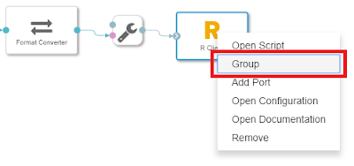
To execute this code SAP Data Hub still needs to know in which Docker container the code should run. This is specified by creating a so called Group. Right click on the R client and choose “Group”.
This creates a slightly shaded area around the R Client, which represents the group. Select the border of this shaded area and click the icon on the bottom right. This opens the configuration of the group, where you can enter the rforecast tag. When running the graph, SAP Data Hub will use the Docker image with that tag, which includes all the required dependencies for our code. Multiple operators can be placed into such a group, hence the name.
Add another Wiretap to the output port of the R Client and save and run the graph. The forecasts were correctly created!
Write the forecasts to SAP HANA
The forecasts exist now within the graph. We want to write them to the SAP HANA table that we created earlier. Add another SAP HANA client to the graph. The input is connected to the data port now (not sql as before). In its configuration
- Specify the connection that was created in the Connection Management.
- Set the “Input format” to JSON.
- Set the “Table name” to the qualified target table, ie TA01.VEHICLEREGISTRATIONS_FORECAST.
- Specify the names and types of the target table’s columns in “Table columns”. Create these individually with the “Add Item” option.
- SEGMENT NVARCHAR(14),
- MONTH DATE,
- MEASURETYPE NVARCHAR(20),
- MEASURE DOUBLE,
- MEASURELOWER DOUBLE,
- MEASUREUPPER DOUBLE,
- MODEL NVARCHAR(100));
The graph should look very much like this now.
Save and run the graph. The time series are written into the SAP HANA table! Here is a preview of the table in the SAP HANA Modeler.
Terminate the graph
The forecasts are created and written into the target table. All the necessary logic has been executed, yet you can see that the graph is still running.
SAP Data Hub contains a specific operator, to gracefully end a graph, the “Graph Terminator”. This operator cannot just be added to our graph though, as the operators at the end of the graph are called multiple times, once for each country. This means that the Graph Terminator would be called as soon as the first country has been forecasted. The graph could then be terminated before all countries have been dealt with. Hence we need to add a gate keeper that calls the Graph Terminator only once all countries have been processed.
Start by calculating the number of countries in the dataset. We want to have this dynamic so that the graph still works well in case the number of countries is changing over time. Add a “1:2 Multiplexer” in front of the current JavaScript operator. This opens up a second branch in the graph.
Continue the new branch with a second “Blank JavaScript” operator. Add one input port called “input” of type string and an output port called “output” of type int64.
This operator will be called only once. Enter the following code, which calculates the number of countries and passes that value to its output port.
$.setPortCallback("input",onInput)
function onInput(ctx,s) {
var json = JSON.parse(s);
$.output(json.length)
}
Add a further Blank JavaScript opreator, which acts as gatekeeper with these three ports
◈ Input port of type int64 called “inputtarget”
◈ Input port of type message called “inputcurrent”
◈ Output port of type string called “output”
Connect the two open branches to the new operator.
Enter the following script into the new JavaScript operator. It is receiving the number of time series that are to be forecasted and it keeps track of how many have already been completed. Once all time series have been processed the graph’s execution continues on the output port. Any value could be passed to the output port, the string itself does not have any meaning or purpose.
$.setPortCallback("inputtarget",onInputTarget)
$.setPortCallback("inputcurrent",onInputCurrent)
var target = -1
var current = 0
function onInputTarget(ctx,s) {
target = s
if (current == target) {
$.output("DONE")
}
}
function onInputCurrent(ctx,s) {
current++
if (current == target) {
$.output("DONE")
}
}
Now only the “Graph Terminator” needs to be added. Run the graph and we are done!
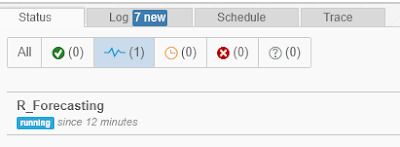
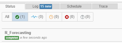
The forecasts have been produced and written into the target table. And the graph has successfully ended. In the status bar it correctly moved from the “Running Graphs” section to the “Completed Graphs” section.
The graph is now independent could be scheduled to regularly produce the latest forecasts.

